


In this article, I will propose an approach to generate natural 2D patterns, like chemical reactions or smoke using a variation of Diffusion-Limited Aggregation (DLA). With this technique, the aggregation of particles does not remain static over time thus opening the way for evolving patterns. A part of the implementation will be done within Processing for educational purposes.
1. Diffusion-Limited Aggregation, a quick overview
The DLA is a process where particles move randomly because of a Brownian motion and cluster together to form aggregates of such particles. A possible algorithm to simulate such phenomena in 2D can be described as following:
- a grid will be used to store the aggregation: it is initialized with zeros and a small area is fed with 1. This area will be the first aggregate
- the particles are distributed in the space, usually at a long distance from the aggregate to prevent weird growth
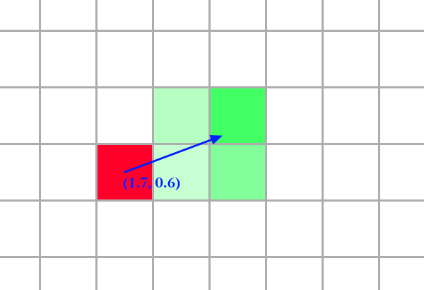
- at each new iterations, each particle is moved to one of its 8 neighbors. If at least one of its neighbors is an aggregate, we set the aggregation map to 1 under the particle position. In other words, if a particle hits the aggregate, it gets added to it
- if a particle was added to the aggregate, it gets removed
This is a simple algorithm. The following illustration shows a possible outcome of this algorithm from the beginning of the generation to the end.
Notice that the initial aggregate is a line in the middle, and particles are introduced at the top and the bottom to create a nicely distributed growth.
2. Introducing the generation of cyclic patterns
The algorithm described in part 1 can only simulate the growth of a finite structure. There are a few things that we can do to allow for a more dynamic behavior, with a dynamic aggregate that can change over time.
First thing, decay of the aggregation can be introduced. At each iteration, every value of the aggregation grid gets multiplied by the decay. Because of the decay, we need to change the distribution of the particles. If they are far away from the first aggregate, they will never be able to hit it before it fades out. So let’s have the particle positions randomized within the whole grid. Also, after a particle hits the aggregate, we will write 1 to the aggregation map at the particles position and reassign a random position to the particle.
We can already observe an interesting behavior: structures keep evolving. We can also observe that over time, the aggregate gets smaller and smaller until it fades out. This is due to the fact that we add a particle to the aggregate if the sum of the neighbors  around the particle is equal or greater than 1. But because of the decay, cases where this condition is true are rarer. This can be solved by introducing an Aggregation threshold
  . If
. If  , then we add the particle to the aggregate.
A last issue remains: what happens if a particle should be added to the aggregate given the sum of its neighbors, but already stands on some aggregate ? It still gets added to it. That’s why the aggregation map gets filled over and over in this case. By preventing aggregation from happening if the value in the aggregation map at a given particle position is higher than a Limitation threshold  , we ensure that the aggregate at this position needs to first decay before it can become 1 again.
Because of this new addition, we can now observe a cycle in the aggregation. This is the very basis of this algorithm. By tweaking the rules of DLA this way, it opens the way some sort of cyclic reaction to happen, a backbone for the generation of even more interesting effects !
The implementation of this system on Processing up to this point is available on Github, you will find the link at the end of the article.
3. Scaling this system up
Due to some limitations of Processing, using Compute shaders isn’t yet supported in the environment (at least not from my research), so I implemented this algorithm at a bigger scale in TouchDesigner. I also think this software is better suited when you work on visuals with precision, I’ve implemented the Processing version just to have something that would appeal to more people. Compute shaders are a way to utilize the graphic card for computations, and I often use them to scale systems up. By having all the particles update done in parallel, you can have millions of them running in real time.
The following illustration demonstrates how the same algorithm performs with this settings:
| Grid size | Particles Nb | Decay | | |
| 900×900 | 230400 | 0.95 | 0.8 | 0.001 |
With a larger grid, more interesting patterns can emerge, and we truly can see how cyclic this system is.
| Grid size | Particles Nb | Decay | | |
| 900×900 | 360000 | 0.9 | 1.2 | 0.001 |
With this set of values, the emerging patterns reminds me of the Belousov-Zhabotinsky reaction [3].
On a side note, I would like to point out the fact that as the ratio particles / grid cells gets closer to 1, basically any cell of the grid can be subject to aggregation. Therefore, it is possible to simulate the same effect without particles, just by considering that a cell has a certain chance to “aggregate” at each iteration. I wrote this on ShaderToy if you are interested by a possible implementation of this idea:
We will stick with particles though, we will later see that this system can be manipulated by playing with the motion of the particles.
4. Applying spatial distortions to the aggregate
Right now, the aggregate is dynamic but it remains static. The motion in the patterns comes from a sweet balance between all the parameters, but we could totally introduce some other distortions and see what happens. Let’s start with a blur. After each iteration, we will apply a 5×5 gaussian blur to the grid of the aggregate.
| Grid size | Particles Nb | Decay | | |
| 900×900 | 193600 | 0.98 | 0.085 | 0.01 |
Unfortunately with this system, I couldn’t find a way to have perfect values that works fine under every condition. It usually requires a bit of trial and error to find something that works well when you introduce a new idea to the system.
Another possibility is to add displacement. Displacement is a way to move individual pixels of a texture to a different position on another texture. A 2D vector field can be used to tell where should the pixels of a texture be picked from another texture. When using GLSL and working with textures, it is not mandatory to use discrete coordinates, for instance it is possible that the output pixel of a texture gets its value grabbed and interpolated from 4 different pixels of an input, if the displacement vector of such pixel isn’t an integer (assuming we are in pixel coordinates).
By using this, we can create a tiny blur which in my opinion can make the effect more organic over time. I will be using some Perlin Noise as a displacement field and make it evolve over time. In the following illustration, I layered the noise used for the displacement on top. Red and Green are used to encode the value of the vector of the displacement field.
| Grid size | Particles Nb | Decay | | |
| 900×900 | 193600 | 0.98 | 0.21 | 0.01 |
We can observe how the displacement influences the reaction. By moving the aggregate, it is more likely that such aggregate will encounter some particles. Thus, the Aggregation Threshold can be increased to prevent a chaotic reaction.
We can think of many other transformations and effects to add at this step. For instance, I tried to add some translation (there is only translation):
| Grid size | Particles Nb | Decay | | |
| 900×900 | 193600 | 0.97 | 0.3 | 0.005 |
Scaling down (0.991):
| Grid size | Particles Nb | Decay | | |
| 900×900 | 193600 | 0.97 | 0.1 | 0.04 |
Rotation:
| Grid size | Particles Nb | Decay | | |
| 900×900 | 193600 | 0.97 | 0.2 | 0.01 |
Be creative and combine what you know to get your own results 
5. Local control of the aggregation rules
Among the 5 parameters affecting the reaction, one of them plays a crucial role: the Aggregation threshold. By itself, it can control… if reaction is happening or not. The other settings are also important, but by tweaking solely the , we can control the whole reaction.
What if we were using a 2D grid, aka a texture, in which we would encode the value of at a particular location ? We would know if aggregation can happen by sampling this texture. In the following illustration, I layered the threshold map, in red, with the reaction. The red component encodes , keep in mind that I lowered the opacity so that the red value does not represent the actual value of , however it gives us an understanding of the variations of between different areas.
We can even have a threshold map that changes over time:
And use the edges of a texture to guide the reaction and the patterns:
Again, this new layer opens many possibilities for interesting ideas and explorations of this system. The other parameters could also be encoded in the texture in the same manner. Feel free to try it out.
6. Moving the particles
By tweaking how the particles move, it is also possible to manipulate the reaction. By having them flow in one direction only, we can force the reaction to happen in the opposite direction. In the next illustration, particles are forced to move to the right only, thus the reaction goes to the left.
Many more things can be done, but I think this is enough for the scope of this article. I really hope you will enjoy playing with this system. You will find a Processing implementation at the end of the article. Comment if you would like the .toe file, I don’t know if it can be useful in such a case.
7. Some more exploration with the system
Follow me on instagram for more content
8. Processing implementation
The source code of the implementation of part 1 and 2 is available on github:
References
- Diffusion-Limited Aggregation, Wikipédia
- Diffusion-Limited Aggregation, Softology’s blog
- Compute Shader, Knonos
- Recreating one of the weirdest reactions (Belousov Zhabotinsky), Tim Kench


